Plotting Early Post-Colonial Elections
In this example, we’ll explore how to visualize early U.S. elections using PoliSciPy. The political landscape of the United States has evolved significantly since its founding, with early elections featuring fewer states and different boundaries compared to today. PoliSciPy enables you to recreate these historical maps, providing insights into the nation’s early electoral geography.
Understanding Early U.S. Elections
After gaining independence, the United States conducted its initial elections with a limited number of states, primarily the original thirteen colonies and a few additional territories. State boundaries and compositions have changed over time; for instance, Massachusetts once included what is now Maine, and Georgia encompassed areas that are currently Alabama and Mississippi. Visualizing these early elections requires accurate historical data and adaptable mapping tools.
Step 1: Install PoliSciPy
Ensure that PoliSciPy is installed on your system. You can install it using pip:
pip install poliscipy
For more installation options and details, refer to the Installation page.
Step 2: Import Necessary Libraries
Once you have PoliSciPy installed, begin by importing it and its relevant methods:
import poliscipy

from poliscipy.shapefile_utils import load_shapefile
from poliscipy.plot import plot_electoral_map
Step 3: Load in the Shapefile
PoliSciPy provides a method for easily loading in shapefiles that contain historical election data. For early elections, it’s crucial to use shapefiles that accurately represent the state boundaries of the specific election year. PoliSciPy includes shapefiles for various historical periods. Load the appropriate shapefile as follows:
gdf = load_shapefile(year="1796")
This function loads a GeoDataFrame containing the geometries and attributes of states as they existed in 1796.
Step 4: Prepare Election Data
Next, prepare the election data corresponding to the chosen year. For the 1796 election, we’ll start by creating a dictionary with the election results:
winning_party_1796 = {
    'CT': 'Adams', 'DE': 'Adams', 'GA': 'Jefferson','KY': 'Jefferson', 'MA': 'Adams','NH': 'Adams',
    'NJ': 'Adams','NY': 'Adams','NC': 'Jefferson','PA': 'Jefferson','RI': 'Adams','SC': 'Jefferson',
    'TN': 'Jefferson','VT': 'Adams','VA': 'Jefferson', 'MD': 'Adams', 'WV': 'Jefferson', 'MS': 'Jefferson',
    'AL': 'Jefferson', 'OH': 'Territories', 'MI': 'Territories', 'WI': 'Territories', 'IL': 'Territories',
    'IN': 'Territories', 'ME': 'Adams'
}
This dictionary includes the states that participated in the 1796 election and the party that won in each state.
Note: In the data dictionary above we have added a category for
Territoriesabove. Note: for representing territories, we can simply create another field in out data dictionary forTerritoriesand then add this to the colormap.
Since we have added a new category Territories to our electoral college map, we need to make sure that we also specify a color in our color map so that PoliSciPy knows which color you would like to use to represent them. For representing territories, it can be useful to show them simply as grey so that they do not get confused with the No Data category.
Create a custom colormap like the one below:
custom_colors_1796 = {
    'Jefferson': '#4397f7',
    'Adams': '#86b97d',
    'No Data': 'lightgrey',
    'Territories': 'grey'
}
Step 5: Merge Election Data with Shapefile
To visualize the election results, merge the election data with the GeoDataFrame:
# add the winning party and fill any missing data with 'No Data'
gdf['winning_party'] = gdf['STUSPS'].map(winning_party_1796).fillna('No Data')
This merges the election results into the GeoDataFrame based on the state names.
Step 6: Add the defecting voters to represent the split states
Adding the defecting voters to represent split states:
# add the number of defecting voters for each respective state
gdf.loc[3, 'defectors'] = 1
gdf.loc[1, 'defectors'] = 1
gdf.loc[18, 'defectors'] = 1
gdf.loc[37, 'defectors'] = 4  # Maryland

# add the defecting party for each of the defecting voters
gdf.loc[3, 'defector_party'] = 'Adams'
gdf.loc[1, 'defector_party'] = 'Adams'
gdf.loc[18, 'defector_party'] = 'Adams'
gdf.loc[37, 'defector_party'] = 'Jefferson'
Step 7: Plot the Electoral Map
With the merged data and defecting voters set, you can now plot the electoral college map:
plot_electoral_map(gdf, column='winning_party', legend=True, party_colors=custom_colors_1796,
                   title="Election of 1796 - Adams vs Jefferson", year=1796)
This function generates a map visualizing the 1796 election results, coloring each state based on the winning party.
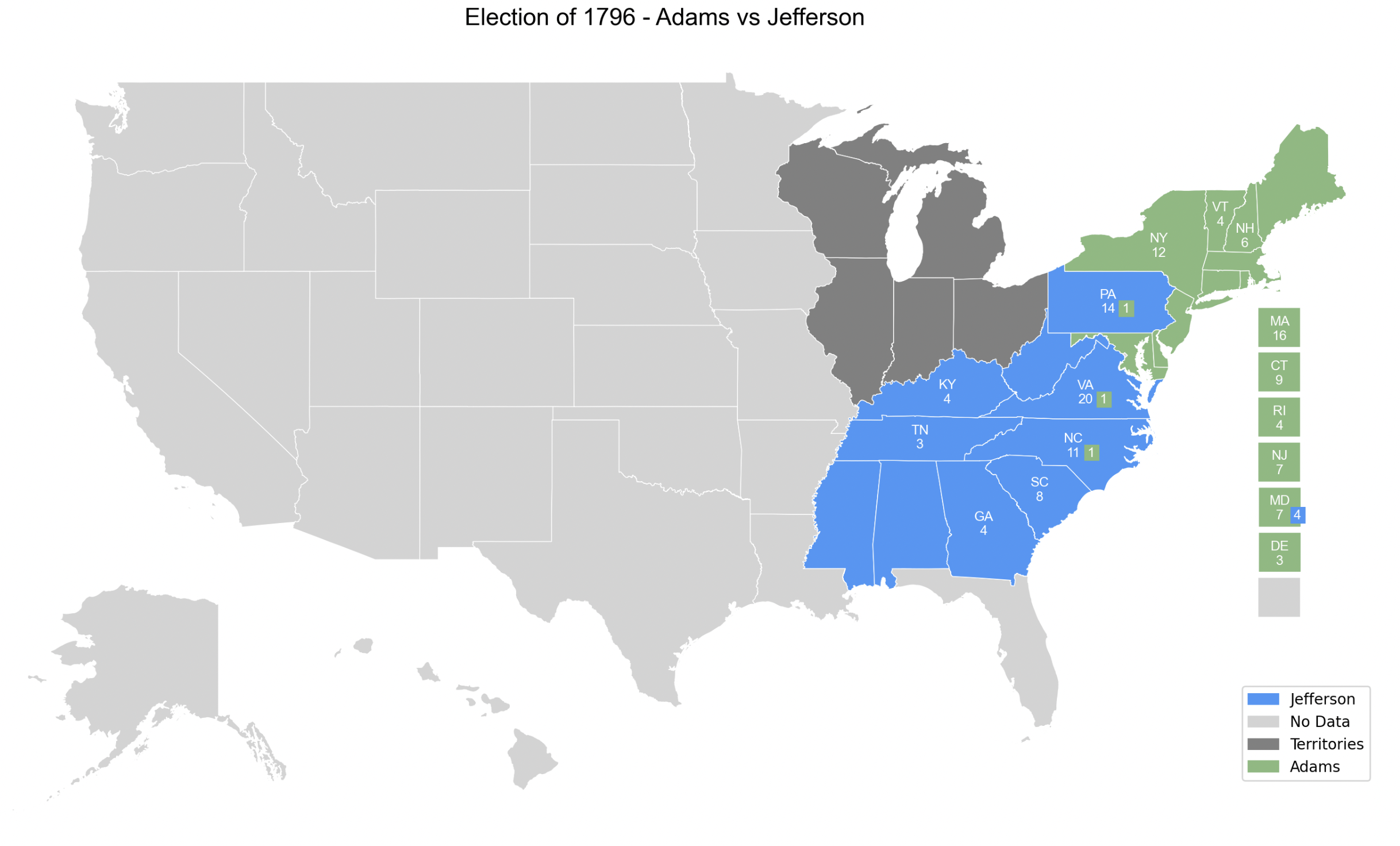
Example Output
Here’s what the 1796 U.S. Presidential Election map should look like after following the steps above: